From Animal Dexterity to Predictive Control: How Modern Robots Sense, Move, and Learn

Introduction

By 2025, robotics has entered a period of unusually rapid expansion. Progress in artificial intelligence, sensing, and computing has pushed robot systems far beyond fixed, preprogrammed execution. What used to be mainly automation is increasingly becoming intelligent autonomy. To understand that shift, it helps to look at the field as an integrated stack: perception, planning, control, learning, and the mechanics that tie them together.

Manipulation begins with biology

Dexterous manipulation and intelligence often appear together in nature. Species with specialized appendages—primate hands, elephant trunks, octopus arms, or the beaks of corvids—tend to show stronger problem-solving ability, more flexible tool use, and better adaptation to changing environments. The relationship is not universal, but complex manipulation and cognition frequently co-evolve and reinforce one another.

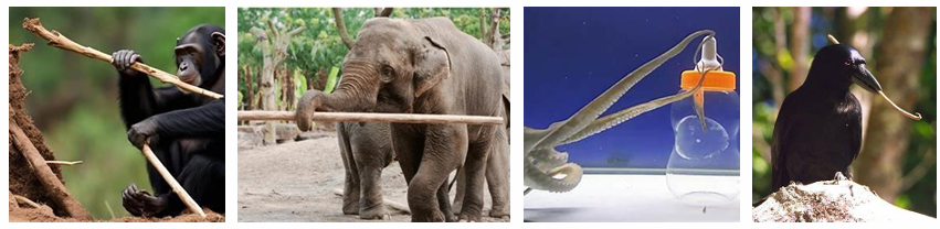
Animals commonly recognized for high intelligence include:

• Chimpanzees
• Dolphins
• Octopi
• Elephants
• Orangutans
• Crows

Octopi are especially striking because roughly 60–70% of their neurons are distributed in peripheral ganglia rather than centralized in the brain, giving them a neural architecture unlike that of most other highly intelligent animals.

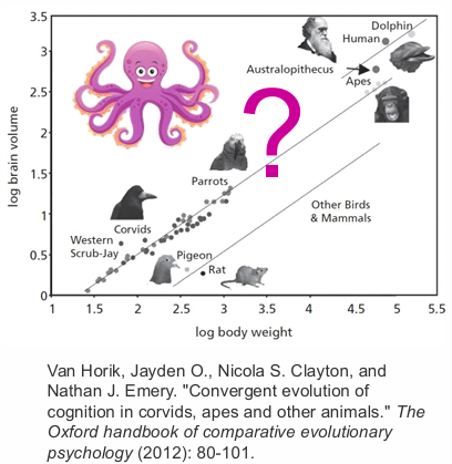
The usual comparison of brain volume to body weight works reasonably well across many species, but octopi remain an outlier: highly capable, yet not well described by the same brain-to-body scaling logic.

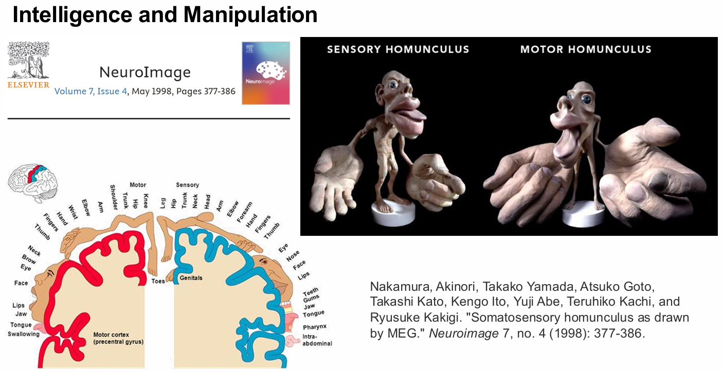
Another biological clue comes from the cortical “homunculus.” In both sensory and motor cortex, body parts such as the hands, lips, and tongue occupy disproportionately large regions. That exaggeration is not accidental—it reflects the importance of fine sensing and precise control.

The language of rigid-body motion

At the core of robot motion lies rigid-body kinematics. Orientation is represented by a rotation matrix $ R \in SO(3) $, a $ 3 \times 3 $ orthogonal matrix satisfying:

$$ R^\top R = I, \quad \det(R) = 1 $$

A rigid body in 3D has three rotational degrees of freedom, corresponding to rotation about the x, y, and z axes.

Position and linear velocity are related by:

$$ \dot{p} = v $$

For orientation, the time evolution of the rotation matrix is tied to angular velocity $ \omega \in \mathbb{R}^3 $ through:

$$ \dot{R} = R [\omega]_\times $$

with the skew-symmetric matrix

$$ [\omega]_\times = \begin{bmatrix} 0 & -\omega_z & \omega_y \ \omega_z & 0 & -\omega_x \ -\omega_y & \omega_x & 0 \end{bmatrix} $$

A full rigid-body pose is written as

$$ g = (R, p) \in SE(3) $$

and its motion can be compactly described by the twist

$$ V = \begin{bmatrix} v \ \omega \end{bmatrix} \in \mathbb{R}^6 $$

This combines translational and rotational velocity into a single object. Intuitively:

• the inertial frame is the fixed world frame,
• the body frame moves with the rigid body,
• $g = (R, p)$ tells us where the body is and how it is oriented,
• $V = [v; \omega]$ describes how it is moving at that instant.

Poisson’s formula and angular velocity

A useful bridge between moving coordinate axes and angular velocity is Poisson’s formula:

$$ \dot{e}_i = \omega \times e_i $$

It says that the time derivative of each axis fixed in the body frame equals the cross product of the angular velocity with that axis. From this, angular velocity can be recovered as:

$$ \omega = (\dot{e}_2 \cdot e_3) e_1 + (\dot{e}_3 \cdot e_1) e_2 + (\dot{e}_1 \cdot e_2) e_3 $$

where $ \dot{e}_i $ is the rate of change of each axis, “·” denotes the dot product, and “×” the cross product. This relation is one of the standard links between the derivative of a rotation matrix and the physical angular velocity vector.

Robot arm architectures

Robot manipulators are typically grouped into serial, parallel, and hybrid structures.

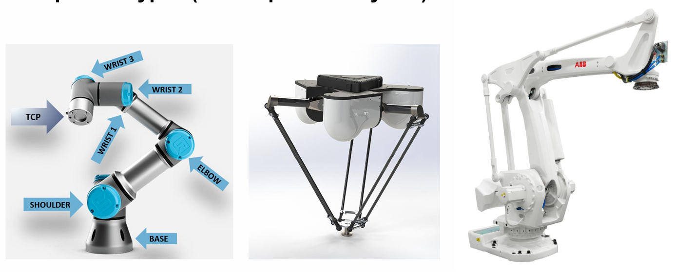
Serial manipulators

Common examples include UR arms and collaborative robots.

• Joints are connected one after another.
• End-effector freedom is built by accumulating joint motions.
• Strengths: large workspace, geometric flexibility, good for complex paths.
• Weaknesses: lower stiffness, accumulated error, slower dynamic response.

Parallel manipulators

Typical examples are Delta robots and high-speed pick-and-place systems.

• The end-effector is driven by multiple kinematic chains.
• The structure forms a closed loop.
• Strengths: high stiffness, low moving mass, high acceleration.
• Weaknesses: smaller workspace and more difficult kinematic analysis.

Hybrid manipulators

Seen in many industrial systems for transport, assembly, spraying, or welding.

• Combine serial and parallel features.
• Strengths: balance of rigidity and flexibility, high payload over a relatively large range.
• Weaknesses: structural complexity, higher cost, harder control design.

A simple summary captures the trade-off well: serial systems are flexible but compliant, parallel systems are stiff and fast, and hybrid systems sit in between while remaining powerful.

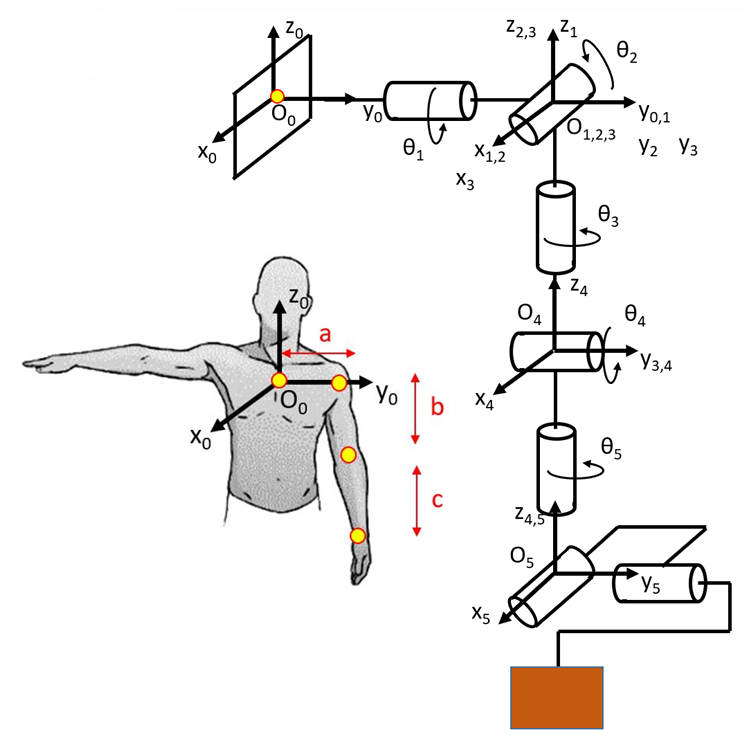
Why the human arm is a useful robot model

The elbow is often idealized as a one-degree-of-freedom revolute joint. In that abstraction, the upper arm and forearm become two rigid links rotating about a common axis.

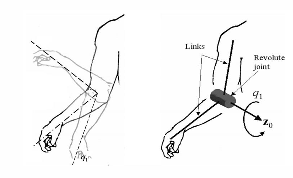
The mapping is straightforward:

• upper arm → Link 1
• forearm → Link 2
• elbow → revolute joint
• joint variable → $ q_1 $
• rotation axis → $ z_0 $

The rotation of the forearm can be written as

$$ \mathbf{R}(q_1) = \begin{bmatrix} \cos q_1 & -\sin q_1 & 0 \ \sin q_1 & \cos q_1 & 0 \ 0 & 0 & 1 \end{bmatrix} $$

This is a standard rigid rotation and one of the building blocks behind DH-style kinematic modeling.

Joint space and workspace

Robot motion can be described in two complementary spaces.

Joint space

Joint variables such as

$$ q_i, \ \theta_i, \ d_i $$

define the robot’s internal configuration.

• $ q_i $: generic joint variable
• $ \theta_i $: angle of a revolute joint
• $ d_i $: displacement of a prismatic joint

The vector $ \mathbf{q} = [q_1, q_2, …, q_n]^\top $ describes a point in joint space.

Workspace

The end-effector’s pose in physical space is described using

$$ p_i(x, y, z), \quad R_i(p_i, p_j, p_k) $$

where position and orientation are represented separately.

Forward kinematics

The mapping from joint coordinates to end-effector pose is

$$ f: \text{Joint Space} \rightarrow \text{Workspace} $$

that is,

$$ (p_i, R_i) = f(q_1, q_2, \dots, q_n) $$

This is forward kinematics: turning internal joint variables into an external position and orientation.

A useful way to say it is:

• joint space describes how the robot moves,
• workspace describes where that motion places the end-effector.

Grasping and force closure

A grasp has force closure when the contacts between a hand or gripper and an object can generate arbitrary net force and torque—collectively, a wrench—so that the object can resist any external disturbance and remain immobilized.

That means, in practical terms, the object stays fixed no matter how it is pushed, pulled, or twisted. Whether force closure is achieved depends on:

• where the contact points are,
• the friction properties at those contacts.

At each contact, feasible contact forces must lie inside a friction cone. A force-closure grasp requires the combined directions spanned by the friction cones to cover the full six-dimensional wrench space: arbitrary forces and arbitrary torques.

This differs from form closure:

• Form closure relies on geometry alone; the object is kinematically trapped and friction is not required.
• Force closure relies on friction plus contact forces to prevent motion.

Minimal contact counts matter:

• In 2D, 2 frictional contacts are sufficient.
• In 3D, at least 4 frictional contacts or 7 frictionless contacts are required.

Why 4 and not 3 in 3D? Because a 3D rigid body has 6 degrees of freedom—three translational and three rotational—and too few contacts cannot span the full 6D wrench space. With friction, each contact can contribute multiple independent components; without friction, each contact contributes only a normal force direction, so more contacts are needed.

Rigid-body dynamics and Newton–Euler equations

The Newton–Euler equations describe both translation and rotation of a rigid body, including robot links.

For translation:

$$ m \ddot{\mathbf{r}}G = \sum \mathbf{F} $$}

For rotation:

$$ I_G \dot{\omega} + \omega \times (I_G \omega) = \sum \tau_{G,\mathrm{ext}} $$

These express two basic laws:

• net force determines center-of-mass acceleration,
• net torque determines the rate of change of angular momentum.

In manipulator dynamics, they form the backbone of recursive force and torque propagation from one link to the next.

Data-driven control without full analytical models

Not every robot is easy to model. Soft robots and strongly nonlinear systems often resist compact analytical descriptions, which makes non-model-based control attractive.

One example is a hybrid controller combining recurrent neural networks and kinematic structure. In work reported in IEEE RA-L, IROS 2024 by a team at EPFL led by Dr. Josie Hughes, with PhD researcher Zixi Chen, an RNN/LSTM module learns nonlinear dynamics online while a kinematic module preserves geometric feasibility and reachability.

The pipeline is:

1. desired trajectory as input,
2. an LSTM that learns dynamic and nonlinear behavior,
3. a kinematic module that enforces geometric consistency,
4. a weighted control output applied directly to the robot.

The method is notable for:

• high open-loop precision without a full physical model,
• large compliant workspace motion,
• natural adaptation to disturbances and contact,
• online learning that improves robustness.

Learning from demonstrations

Imitation learning teaches robots by having them observe demonstrations rather than by hand-coding rewards or exhaustive task rules.

A robot learns a policy $ \pi(a|s) $ so that in a state $ s $ it chooses an action $ a $ similar to what a human would do in that situation.

Important data sources include:

• instructional and how-to videos from online platforms,
• first-person datasets such as Ego4D,
• visual and manipulation representation systems such as R3M, MVP, and Voltron.

Large-scale real-world robot imitation efforts include ArmFarm, RT1, RT2, and collaborative datasets such as Open-X Embodiment and DROID, which collectively span more than 20 institutions, 22 robot embodiments, 500+ skills, and 60+ datasets.

Simulation remains central as well. Platforms such as ManiSkill, Orbit, and Isaac Sim support high-fidelity task learning and evaluation, while RoboTurk and MimicGen provide teleoperated demonstration data and support combined imitation-learning and reinforcement-learning pipelines.

The core idea is simple: robots watch humans act, then learn to act on their own.

Differential kinematics and the Jacobian

Differential kinematics connects joint velocities to end-effector motion:

$$ \mathbf{v} = \mathbf{J(q)} \cdot \dot{\mathbf{q}} $$

Here,

• $\mathbf{q} \in \mathbb{R}^n$ is the joint configuration,
• $\dot{\mathbf{q}} \in \mathbb{R}^n$ is the joint-velocity vector,
• $\mathbf{v} \in \mathbb{R}^6$ is the end-effector twist,
• $\mathbf{J(q)} \in \mathbb{R}^{6 \times n}$ is the Jacobian.

The Jacobian is the velocity bridge between joint space and workspace. Each column tells us how one joint, moving at unit speed, contributes to the end-effector’s linear and angular velocity.

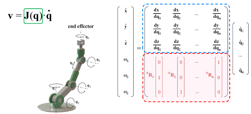
It is commonly partitioned as

$$ \mathbf{J} = \begin{bmatrix} \mathbf{J}v \ \mathbf{J}\omega \end{bmatrix} $$

with

• $\mathbf{J}_v$ mapping joint rates to linear velocity,
• $\mathbf{J}_\omega$ mapping joint rates to angular velocity.

The rotational component can be written as the sum of joint-axis contributions:

$$ {}^{0}\omega_{6/wrt,0} = {}^{0}\mathbf{R}_1 \hat{\mathbf{z}}_1 \dot{q}_1 + {}^{0}\mathbf{R}_2 \hat{\mathbf{z}}_2 \dot{q}_2 + {}^{0}\mathbf{R}_3 \hat{\mathbf{z}}_3 \dot{q}_3 + {}^{0}\mathbf{R}_4 \hat{\mathbf{z}}_4 \dot{q}_4 + {}^{0}\mathbf{R}_5 \hat{\mathbf{z}}_5 \dot{q}_5 + {}^{0}\mathbf{R}_6 \hat{\mathbf{z}}_6 \dot{q}_6 $$

The Jacobian also appears in:

• velocity control: $\dot{\mathbf{q}} = \mathbf{J}^{-1}\mathbf{v}$,
• force mapping: $\boldsymbol{\tau} = \mathbf{J}^T \mathbf{F}$,
• singularity analysis, when $\det(\mathbf{J}\mathbf{J}^T) = 0$,
• redundancy resolution using the pseudoinverse $\mathbf{J}^+$ when $n > 6$.

Inverse Jacobian motion control

If the desired end-effector velocity is known and the task is to recover the required joint rates, the inverse Jacobian gives the reverse mapping:

$$ \dot{\mathbf{q}} = \mathbf{J}^{-1}(\mathbf{q}) \cdot \mathbf{v} $$

In practice, this is used iteratively for position control: from an initial position to a target position, the direction, distance, and execution time define a desired Cartesian velocity, and integrating the resulting joint rates produces the motion.

The same logic extends to orientation control. If the initial and target rotation matrices are $R_i$ and $R_f$, and the execution time $t_f$ is known, the required angular-velocity component of the twist can be computed from the relative rotation.

For a rotation matrix

$$ R = \begin{bmatrix} a & b & c \ d & e & f \ g & h & i \end{bmatrix} $$

a corresponding rotation vector is

$$ \mathbf{u} = \begin{bmatrix} h - f \ c - g \ d - b \end{bmatrix}, \quad |\mathbf{u}| = 2 \sin \theta $$

When the Jacobian is not invertible—either because the manipulator is redundant or because it is near a singularity—the Moore–Penrose pseudoinverse is used:

$$ \mathbf{J}^{+} = \mathbf{J}^T (\mathbf{J}\mathbf{J}^T)^{-1} $$

and then

$$ \dot{\mathbf{q}} = \mathbf{J}^{+}(\mathbf{q}) \cdot \mathbf{v} $$

Square, slim, and fat Jacobians

Since the task-space twist is six-dimensional, the Jacobian always has shape $6 \times n$. That leads to three important cases:

• $n < 6$: under-actuated, typically no exact 6D solution,
• $n = 6$: fully actuated, square Jacobian, unique exact solution when nonsingular,
• $n > 6$: redundant, infinitely many solutions.

This leads to the useful shape classification:

• Square Jacobian: $N = 6$, common in six-axis industrial arms, directly invertible when nonsingular.
• Slim Jacobian: $N < 6$, under-actuated, often seen in planar or task-limited systems like SCARA.
• Fat Jacobian: $N > 6$, redundant systems with null-space freedom, common in flexible, snake-like, or continuum robots.

For non-square cases, pseudoinverse solutions are used. In the under-actuated case, one seeks to minimize joint-speed norm; in the redundant case, one typically minimizes end-effector tracking error in a least-squares sense.

State-space representation

Modern control describes systems through first-order differential equations in state-space form:

$$ \dot{x}(t) = A x(t) + B u(t) $$ $$ y(t) = C x(t) + D u(t) $$

where:

• $x(t)$ is the state vector,
• $u(t)$ the input,
• $y(t)$ the output,
• $A, B, C, D$ are system, input, output, and direct feedthrough matrices.

This framework is useful because it captures internal system memory—position, velocity, current, and so on—rather than just an input-output relation. It works for both SISO and MIMO systems and provides the mathematical basis for controllability, observability, state feedback, LQR, and many other control methods.

Nonlinear systems and linearization

Most real robotic, mechanical, electrical, and biological systems are nonlinear. A pendulum already shows this clearly:

$$ m l^2 \ddot{\theta} + b \dot{\theta} + m g l \sin(\theta) = T $$

Robot dynamics are even more nonlinear, with trigonometric and coupling terms throughout. The difficulty is that many standard analytical tools—transfer functions, root locus, frequency response—are designed for linear systems.

The usual solution is local linearization. Given

$$ \dot{x}(t) = f(x(t), u(t)), \quad y(t) = g(x(t), u(t)) $$

one linearizes around a working point $(x^{sol}, u^{sol})$ to obtain

$$ \delta \dot{x}(t) = A(t)\,\delta x(t) + B(t)\,\delta u(t) $$ $$ \delta y(t) = C(t)\,\delta x(t) + D(t)\,\delta u(t) $$

with Jacobians

$$ A(t) = \frac{\partial f}{\partial x}(x^{sol}, u^{sol}), \quad B(t) = \frac{\partial f}{\partial u}(x^{sol}, u^{sol}) $$

$$ C(t) = \frac{\partial g}{\partial x}(x^{sol}, u^{sol}), \quad D(t) = \frac{\partial g}{\partial u}(x^{sol}, u^{sol}) $$

Linearizing about an equilibrium $(x^{eq}, u^{eq})$ where $f(x^{eq}, u^{eq}) = 0$ yields an LTI model:

$$ \delta \dot{x}(t) = A \delta x(t) + B \delta u(t) $$ $$ \delta y(t) = C \delta x(t) + D \delta u(t) $$

This is central in robotics because it enables practical controller design near a nominal posture or trajectory.

Feedback linearization

Linearization by approximation is one route. A more aggressive route is feedback linearization, which cancels the system’s nonlinearities directly through the control law.

For

$$ \dot{x} = f(x) + g(x)u, \quad y = h(x) $$

one introduces

$$ u = \alpha(x) + \beta(x)v $$

so that the closed-loop system behaves like a linear one:

$$ \dot{x} = A x + B v $$

The basic idea is:

• choose $\alpha(x)$ to cancel internal nonlinearities,
• choose $\beta(x)$ to normalize the input channel,
• design $v$ using linear control tools such as PID or LQR.

For robot dynamics,

$$ M(q)\ddot{q} + B(q, \dot{q})\dot{q} + G(q) = F $$

one may define

$$ F = u = u_{nl}(q, \dot{q}) + M(q)v $$

with

$$ u_{nl}(q, \dot{q}) = B(q, \dot{q})\dot{q} + G(q) $$

which reduces the dynamics to the double integrator

$$ \ddot{q} = v $$

This is the essence of why feedback linearization is so powerful in robotics.

Stability: from eigenvalues to Lyapunov energy

A control system is useful only if it is stable. Several notions matter.

BIBO stability

A system is BIBO stable if bounded input implies bounded output:

$$ |u(t)| < \infty \quad \Rightarrow \quad |y(t)| < \infty $$

Internal stability in state space

For

$$ \dot{x}(t) = A x(t) + B u(t), \quad y(t) = C x(t) + D u(t) $$

stability is governed by the eigenvalues of $A$:

$$ \Re(\lambda_i(A)) < 0 \quad \forall i $$

• negative real parts → asymptotically stable,
• zero real parts → marginally stable,
• positive real part anywhere → unstable.

Lyapunov stability

For nonlinear systems,

$$ \dot{x} = f(x) $$

a Lyapunov function $V(x)$ acts like an energy measure. If

$$ V(x) > 0 \text{ for } x \ne 0, \quad V(0) = 0 $$

and

$$ \dot{V}(x) < 0 $$

the equilibrium is asymptotically stable.

A simple example is

$$ \dot{x} = -x $$

with

$$ V(x) = x^2 $$

Then

$$ \dot{V}(x) = 2x\dot{x} = 2x(-x) = -2x^2 < 0 $$

so the origin is asymptotically stable.

Transfer functions and Laplace-domain stability

For linear time-invariant systems, the transfer function

$$ G(s) = \frac{Y(s)}{U(s)} $$

encodes the input-output relation in the Laplace domain. Laplace transforms convert differential equations into algebraic ones:

$$ \mathcal{L}[f(t)] = F(s) = \int_0^{\infty} f(t)e^{-st}dt $$

The poles of

$$ G(s) = \frac{N(s)}{D(s)} $$

are the roots of $D(s)=0$, and BIBO stability requires all poles to lie strictly in the left half-plane:

$$ \Re(p_i) < 0 \quad \forall \text{ poles } p_i $$

This is the frequency-domain counterpart to eigenvalue-based internal stability.

Existence and uniqueness of nonlinear solutions

For a nonlinear system

$$ \dot{x} = f(t, x) $$

two mathematical questions matter: does a solution exist, and is it unique?

Existence is supported if $f(t,x)$ is piecewise continuous in time. Uniqueness is guaranteed locally if the function is locally Lipschitz in $x$:

$$ |f(t, x) - f(t, y)| \le L |x - y| $$

within some neighborhood.

Without the Lipschitz condition, uniqueness can fail. A standard example is

$$ \dot{x} = x^{1/3}, \quad x(0) = 0 $$

which admits multiple solutions, including

$$ x(t) \equiv 0, \quad x(t) = \left(\frac{2t}{3}\right)^{3/2} $$

The distinction between local and global Lipschitz continuity also matters. Local Lipschitz continuity gives local uniqueness; global Lipschitz continuity supports global uniqueness. Finite escape time remains possible in locally Lipschitz systems, as in

$$ \dot{x} = -x^2, \quad x(0) = -1 $$

with solution

$$ x(t) = \frac{1}{t - 1} $$

which diverges to $-\infty$ at $t=1$.

Equilibria, phase planes, and local behavior

A point $x^*$ is an equilibrium if, once the system starts there, it stays there. For autonomous systems,

$$ \dot{x} = f(x) $$

equilibria satisfy

$$ f(x) = 0 $$

In two-dimensional systems, phase-plane tools help visualize dynamics:

• the vector field gives local direction and speed,
• nullclines are curves where one state derivative is zero,
• their intersections are equilibria,
• isoclines are curves of constant trajectory slope.

For linear planar systems

$$ \dot{x} = A x, \quad A \in \mathbb{R}^{2\times2} $$

the eigenvalues of $A$ determine local geometry:

• two negative real eigenvalues → stable node,
• two positive real eigenvalues → unstable node,
• opposite signs → saddle,
• complex pair with negative real part → stable focus,
• complex pair with positive real part → unstable focus,
• purely imaginary pair → center.

For nonlinear systems, the Jacobian at an equilibrium gives the linearized local model, so nearby behavior can often be inferred from that same classification.

Limit cycles and self-sustained oscillation

Nonlinear systems can do something linear systems cannot: sustain isolated periodic motion without external forcing. That is the essence of a limit cycle.

A classical example is the Van der Pol oscillator:

$$ \dot{x}_1 = x_2, \qquad \dot{x}_2 = -x_1 + \varepsilon(1 - x_1^2)x_2 $$

with $\varepsilon > 0$ controlling the nonlinear damping. For small $\varepsilon$, the behavior is near-linear; for larger values, the system settles onto a stable closed orbit. Around a limit cycle $\Gamma$, there exists a period $T>0$ such that

$$ x(t + T) = x(t), \quad \forall t $$

Nearby trajectories either converge to $\Gamma$ (stable limit cycle) or diverge away from it (unstable limit cycle). This is one of the canonical nonlinear phenomena missing from linear models.

Model predictive control

Model Predictive Control, or MPC, is built around a simple idea: predict the future using a model, optimize control over a finite horizon, apply only the first control input, then repeat.

At time step $k$, MPC solves

$$ \min_{u_0, \dots, u_{N-1}} \sum_{j=0}^{N-1} \ell(x_j, u_j) + V_f(x_N) $$

subject to

$$ x_{j+1} = f(x_j, u_j), \quad (x_j, u_j) \in \mathcal{X} \times \mathcal{U} $$

and then applies $u_k^ = u_0^$.

In robotics, MPC is attractive because it handles constraints explicitly:

• actuator limits,
• joint, position, velocity, and acceleration bounds,
• safety distances from obstacles.

A standard quadratic cost is

$$ J = \sum_{k=0}^{N-1} |x_k - x_k^{\text{ref}}|_Q^2 + |u_k|_R^2 + |x_N - x_N^{\text{ref}}|_P^2 $$

Tuning $Q$, $R$, and $P$ trades off tracking accuracy, smoothness, and terminal precision.

Linearization and discretization for MPC

MPC is usually implemented in discrete time. A continuous LTI model

$$ \dot{x}(t) = A_c x(t) + B_c u(t) $$

with zero-order hold becomes

$$ x_{k+1} = A x_k + B u_k $$

where

$$ A = e^{A_c T_s}, \quad B = \int_0^{T_s} e^{A_c \tau} B_c \, d\tau $$

Choosing the sampling time $T_s$ is a practical balancing act. If it is too large, aliasing and model mismatch appear; if too small, the optimization burden can exceed real-time limits.

When the underlying robot dynamics are nonlinear,

$$ \dot{x} = f(x, u) $$

one often linearizes locally:

$$ \dot{x} \approx A x + B u + c $$

This allows standard linear MPC to be posed as a convex quadratic program. The linearization may be about an equilibrium, yielding an LTI model, or about a nominal trajectory, yielding an LTV model.

Standard MPC formulation

The standard finite-horizon problem is

$$ \min_{ {u_i}{i=0}^{N-1} } \sum \ell(x_i, u_i) + V_f(x_N) $$}^{N-1

subject to:

$$ \begin{cases} x_{i+1} = f(x_i, u_i), & i = 0, \dots, N-1, \ x_0 = \hat{x}_k, & \text{(current measured state)} \ g(x_i, u_i) \le 0, & \text{(general inequality constraints)} \ h(x_N) \le 0, & \text{(terminal constraint or stability condition)} \ u_i \in \mathcal{U},\; x_i \in \mathcal{X}, & \text{(input and state constraints)} \end{cases} $$

with stage cost

$$ \ell(x, u) = |x - x_{\text{ref}}|_Q^2 + |u|_R^2 $$

and terminal cost

$$ V_f(x_N) = |x_N - x_{\text{ref}}|_P^2 $$

Linear dynamics and quadratic cost reduce the problem to a QP; nonlinear dynamics lead to nonlinear programming.

Typical MPC examples

Three representative examples illustrate the range:

1. Unicycle robot

Continuous kinematics:

$$ \dot{p}_x = v \cos \theta, \quad \dot{p}_y = v \sin \theta, \quad \dot{\theta} = \omega $$

Linearized around near-straight motion and discretized, this becomes a standard linear MPC tracking problem with state and input constraints.

1. 2-DOF robot arm

Dynamics:

$$ M(q)\ddot{q} + C(q, \dot{q})\dot{q} + g(q) = \tau $$

Written in state space and discretized using RK4, this leads to a nonlinear MPC problem solved by methods such as SQP or interior-point optimization.

1. Thermal control system

$$ \dot{T}(t) = -\alpha (T(t) - T_{\text{env}}) + \beta u(t) $$

After discretization:

$$ T_{k+1} = (1 - \alpha T_s)T_k + \beta T_s u_k $$

This becomes a small QP balancing temperature error against energy input.

Model-based dynamic control

Manipulator dynamics are nonlinear because inertia changes with configuration, Coriolis and centrifugal terms depend on motion, and gravity depends on posture. Model-based dynamic control explicitly uses that structure to cancel or compensate the nonlinear terms so that the remaining error dynamics are easier to control.

The general robot dynamics are written as

$$ M(q)\ddot{q} + C(q, \dot{q})\dot{q} + g(q) = \tau $$

The basic motivation is straightforward:

• compensate for nonlinear effects,
• obtain nearly linear error dynamics,
• support Lyapunov-based stability proofs,
• preserve tracking performance under high speed or changing payload.

Computed torque control

Computed Torque Control (CTC) is the classic inverse-dynamics approach. The goal is to force the tracking error

$$ e = q - q_d, \quad \dot{e} = \dot{q} - \dot{q}_d $$

to satisfy a linear second-order equation:

$$ \ddot{e} + K_d \dot{e} + K_p e = 0 $$

This is achieved by choosing

$$ \tau = M(q) v + C(q, \dot{q})\dot{q} + g(q) $$

with

$$ v = \ddot{q}_d - K_d \dot{e} - K_p e $$

Substituting this into the robot dynamics yields the desired linear closed-loop error system. Each joint behaves like a decoupled second-order system whose natural frequency and damping are determined by $K_p$ and $K_d$.

The strengths are clear: fast, accurate, and predictable tracking. The weaknesses are equally clear: heavy reliance on accurate models and sensitivity to modeling error or noise.

Full-state feedback linearization and task-space linearization

CTC is one expression of a broader idea: full-state feedback linearization in joint space. Using the inverse-dynamics law

$$ \tau = M(q)(\ddot{q}_d - K_d \dot{e} - K_p e) + C(q, \dot{q})\dot{q} + g(q) $$

the nonlinear joint-space system becomes

$$ \ddot{e} + K_d \dot{e} + K_p e = 0 $$

A parallel idea works in task space. If the output is

$$ y = h(q) \in \mathbb{R}^m $$

then

$$ \dot{y} = J(q)\dot{q}, \quad \ddot{y} = J(q)\ddot{q} + \dot{J}(q, \dot{q})\dot{q} $$

With a suitable control law, one can force the task-space error $e_y = y - y_d$ to satisfy

$$ \ddot{e}y + K}\dot{ey + K e_y = 0 $$

whenever $J(q)$ is nonsingular. This is more direct for end-effector trajectory control, though it is more sensitive to Jacobian singularities and requires $J$ and $\dot{J}$.

The relative degree here is 2, because the control input appears directly in the second derivative of the output. Once linearized, the same familiar second-order control design logic applies.

Adaptive control and Slotine–Li

Real robots never match their models perfectly. Mass, friction, payload, drag, and other parameters are often uncertain. Adaptive control addresses this by estimating unknown parameters online and updating the control law as the robot moves.

A key assumption is linear parameterization: the uncertain dynamics can be written as a known regressor times an unknown constant parameter vector.

For robot manipulators,

$$ M(q)\ddot{q} + C(q, \dot{q})\dot{q} + g(q) = \tau $$

and there exists a regressor $Y(\cdot)$ such that

$$ M(q)\xi + C(q, \dot{q})\zeta + g(q) = Y(q, \dot{q}, \zeta, \xi)\theta $$

for an unknown constant parameter vector $\theta$.

The Slotine–Li design defines tracking and filtered errors as

$$ e := q - q_d, \quad s := \dot{e} + \Lambda e $$

with reference signals

$$ \dot{q}_r := \dot{q}_d - \Lambda e, \quad \ddot{q}_r := \ddot{q}_d - \Lambda \dot{e} $$

so that

$$ s = \dot{q} - \dot{q}_r, \quad \dot{s} = \ddot{q} - \ddot{q}_r $$

The control law is

$$ \tau = Y(q, \dot{q}, \dot{q}_r, \ddot{q}_r)\hat{\theta} - K_d s $$

and the adaptation law is

$$ \dot{\hat{\theta}} = -\Gamma Y(q, \dot{q}, \dot{q}_r, \ddot{q}_r)^{\top}s $$

with positive definite gains $K_d$ and $\Gamma$.

Substituting into the dynamics yields

$$ M(q)\dot{s} + C(q, \dot{q})s + K_d s = Y(q, \dot{q}, \dot{q}_r, \ddot{q}_r)\tilde{\theta} $$

where $\tilde{\theta} = \hat{\theta} - \theta$ is the parameter estimation error.

A Lyapunov candidate,

$$ V = \frac{1}{2}s^{\top}M(q)s + \frac{1}{2}\tilde{\theta}^{\top}\Gamma^{-1}\tilde{\theta} $$

leads to

$$ \dot{V} = -s^{\top}K_d s \le 0 $$

which establishes boundedness and, using Barbalat’s lemma, convergence of $s(t)$ to zero and thus convergence of the tracking error. The appeal of Slotine–Li is that it preserves stability and tracking without requiring exact parameter knowledge, and it does so without the chattering associated with switching control.

Sliding mode control

When disturbances are large and matched through the input channel, sliding mode control (SMC) offers strong robustness and finite-time convergence to a designed manifold.

Start with the disturbed robot model:

$$ M(q)\ddot{q} + C(q,\dot{q})\dot{q} + g(q) = \tau + d(t) $$

with bounded disturbance components $|d_i(t)| \le \Delta_i$.

Define the tracking and sliding variables:

$$ e := q - q_d, \qquad \dot{e} := \dot{q} - \dot{q}_d $$

$$ s := \dot{e} + \Lambda e, \qquad \Lambda = \Lambda^\top \succ 0 $$

On the manifold $s=0$, the error dynamics reduce to

$$ \dot{e} + \Lambda e = 0 $$

which means the tracking error decays exponentially once the system reaches the surface.

Using the reference signals

$$ \dot{q}_r := \dot{q}_d - \Lambda e,\qquad \ddot{q}_r := \ddot{q}_d - \Lambda \dot{e} $$

one obtains the key balance:

$$ M\dot{s} + C s = (\tau - \tau_{eq}) + d(t) $$

where

$$ \tau_{eq} = M(q)(\ddot{q}_d - \Lambda \dot{e}) + C(q,\dot{q})\dot{q} + g(q) $$

is the nominal equivalent control.

With Lyapunov function

$$ V_s = \tfrac{1}{2} s^\top M(q) s $$

one gets

$$ \dot{V}s = s^\top\big((\tau - \tau) + d\big) $$

The ideal discontinuous SMC law is

$$ u = -K\,\operatorname{sgn}(s), \qquad K=\operatorname{diag}{k_i}\succ 0, $$

so the full control is $\tau = \tau_{eq} + u$. Then

$$ \dot{V}_s = -\sum_i k_i|s_i| + \sum_i d_i s_i $$

and if $k_i > \Delta_i$ for each component,

$$ \dot{V}_s \le -\sum_i (k_i - \Delta_i)|s_i| $$

which guarantees finite-time reaching.

Because ideal switching causes chattering, a practical boundary-layer version replaces the sign function with saturation:

$$ u = -K\,\operatorname{sat}(s/\phi),\qquad \operatorname{sat}(z)=\begin{cases} \operatorname{sgn}(z), & |z|\ge 1, \ z, & |z|<1, \end{cases} $$

and the complete law becomes

$$ \tau = \tau_{eq} - K\,\operatorname{sat}(s/\phi) $$

This removes high-frequency chattering at the cost of a bounded steady-state layer. For even smoother behavior, second-order methods such as super-twisting can be used:

$$ u_i = -k_{1i} |s_i|^{1/2}\operatorname{sgn}(s_i) + v_i,\qquad \dot{v}i = -k(s_i) $$}\operatorname{sgn

which reduce chattering while preserving strong robustness under additional assumptions.

What the control torque does in four common strategies

Across several nonlinear robot controllers, the torque $\tau$ plays a similar structural role—nominal compensation plus a strategy-specific correction term—but the correction mechanism differs.

Joint-space CTC

$$ \tau = M(q)\,v + C(q,\dot{q})\dot{q} + g(q),\qquad v = \ddot{q}_d - K_d\dot{e} - K_p e $$

Here $\tau$ cancels the nominal dynamics exactly and imposes linear second-order tracking error dynamics. Accuracy is high, but robustness depends on model fidelity.

Task-space inverse dynamics

$$ F_{eq} = \Lambda(\ddot{x}d - \Lambda_x \dot{e}_x) + \bar{\Xi}\dot{x} + p,\qquad F = F(s_x/\phi_x) $$} - K_x\operatorname{sat

mapped back to joints as

$$ \tau = J(q)^\top F $$

Now the design happens directly in task space and torque is used as the Jacobian-transposed realization of the desired task-space force.

Slotine–Li adaptive control

$$ \tau = Y(q,\dot{q},\dot{q}_r,\ddot{q}_r)\,\hat{\theta} - K_d s $$

with

$$ \dot{\hat{\theta}} = -\Gamma Y^\top s $$

The torque combines estimated-dynamics compensation with a damping term. The controller learns uncertain parameters online rather than requiring them in advance.

Sliding mode control

$$ \tau_{eq} = M(q)(\ddot{q}_d - \Lambda \dot{e}) + C(q,\dot{q})\dot{q} + g(q) $$

$$ \tau = \tau_{eq} - K\,\operatorname{sat}(s/\phi) $$

Torque first cancels the nominal dynamics, then adds a robust switching or saturation term that drives the system to the sliding manifold despite bounded matched disturbances.

In short:

• CTC relies on exact model cancellation,
• task-space control pushes that cancellation to the end-effector level,
• Slotine–Li replaces exact parameters with online estimates,
• SMC adds a discontinuous or smoothed robust term to overpower disturbances.

Robotic control rarely uses just one idea in isolation. In practice, nominal model compensation is often combined with adaptation, robust terms, or predictive optimization, depending on whether the priority is precision, uncertainty handling, or safety under constraints.