A recent paper used the frequency of Weibo keywords to predict air pollution and argued that social media data can add finer detail to environmental monitoring. That idea is appealing. But if we set aside the environmental angle for a moment, the text-analysis side of Weibo is not especially hard to implement. A simple way to demonstrate that is to test whether a Weibo corpus follows Zipf’s law.
The dataset used here is an open Weibo corpus from NLPIR, containing about 230,000 posts. From that corpus, the goal is to extract words and their frequencies, then check a classic bibliometric pattern: Zipf’s law. In its usual form, if a word’s frequency is (f) and its rank is (r), then their product should be approximately constant:
[ r \times f = C ]
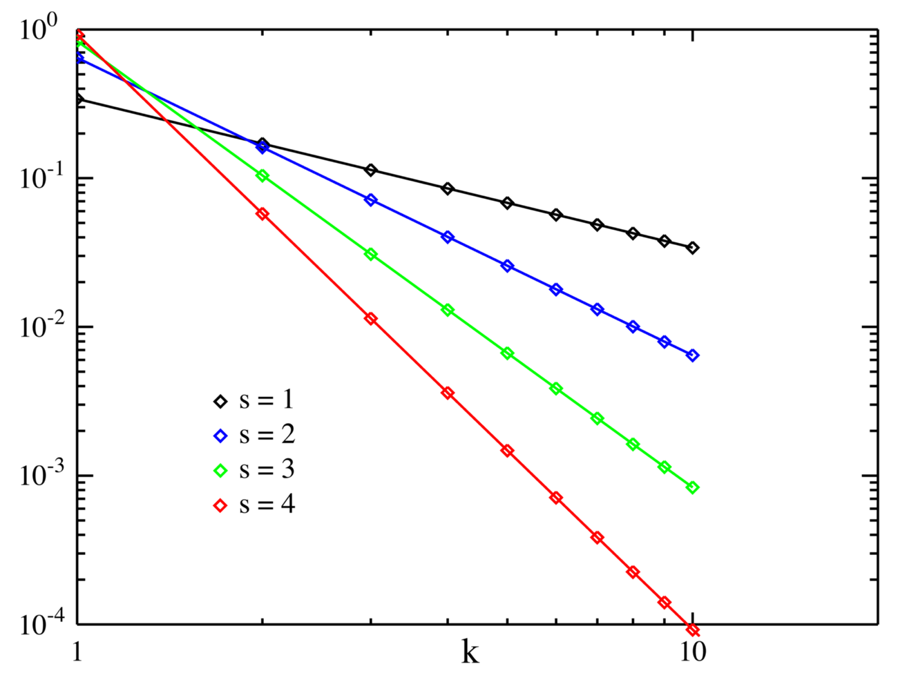
The figure above comes from Wikipedia.
Code used for the analysis
The following code can be reproduced once the dataset has been downloaded and the file path is set correctly.
# 读入xml包
library(XML)
# 读取数据并提取文本信息
doc <- xmlTreeParse('NLPIR微博内容语料库.xml',useInternal=TRUE)
rootNode <- xmlRoot(doc)
doc1 <- xpathSApply(rootNode,"//article",xmlValue)
# 去除无关标点与数字
doc2 <- gsub(pattern="http:[a-zA-Z\\/\\.0-9]+","",doc1)
# 中文分词
library(Rwordseg)
doc3 <- segmentCN(doc2)
# 构建语料库 去掉标点与数字与高频词
library(tm)
doc4 <- Corpus(VectorSource(doc3))
doc5 <- tm_map(doc4, removePunctuation)
doc6 <- tm_map(doc5, removeNumbers)
# 高频无意义词在这里可以搞到 https://github.com/yufree/democode/tree/master/data
x <- scan("stopwords.txt", what="")
doc7 <- tm_map(doc6, removeWords, x)
doc8 <- tm_map(doc7, stripWhitespace)
# 构建全范围的词频矩阵
control=list(minDocFreq=5,wordLengths = c(1, Inf),bounds = list(global = c(5,Inf)),weighting = weightTf,encoding = 'UTF-8')
doc.tdm=TermDocumentMatrix(doc8,control)
# 这里截取词频高于5长度为2的词
control2=list(minDocFreq=5,wordLengths = c(2, 2),bounds = list(global = c(5,Inf)),weighting = weightTf,encoding = 'UTF-8')
doc.tdm2=TermDocumentMatrix(doc8,control2)
# 这里截取词频高于5长度为3的词
control3=list(minDocFreq=5,wordLengths = c(3, 3),bounds = list(global = c(5,Inf)),weighting = weightTf,encoding = 'UTF-8')
doc.tdm3=TermDocumentMatrix(doc8,control3)
# 这里截取词频高于5长度为4的词
control4=list(minDocFreq=5,wordLengths = c(4, 4),bounds = list(global = c(5,Inf)),weighting = weightTf,encoding = 'UTF-8')
doc.tdm4=TermDocumentMatrix(doc8,control4)
# 这里截取词频高于5长度为5的词
control5=list(minDocFreq=5,wordLengths = c(5, 5),bounds = list(global = c(5,Inf)),weighting = weightTf,encoding = 'UTF-8')
doc.tdm5=TermDocumentMatrix(doc8,control5)
# 得到词频列表
library(slam)
freq <- rowapply_simple_triplet_matrix(doc.tdm,sum)
freq2 <- rowapply_simple_triplet_matrix(doc.tdm2,sum)
freq3 <- rowapply_simple_triplet_matrix(doc.tdm3,sum)
freq4 <- rowapply_simple_triplet_matrix(doc.tdm4,sum)
freq5 <- rowapply_simple_triplet_matrix(doc.tdm5,sum)
# save(freq,freq2,doc8,file ='constellation.RData')
# 验证齐普夫定律
order <- order(freq[order(freq,decreasing = T)],decreasing = T)
freq0 <- freq[order(freq,decreasing = T)]
order2 <- order(freq2[order(freq2,decreasing = T)],decreasing = T)
freq20 <- freq2[order(freq2,decreasing = T)]
order3 <- order(freq3[order(freq3,decreasing = T)],decreasing = T)
freq30 <- freq3[order(freq3,decreasing = T)]
order4 <- order(freq4[order(freq4,decreasing = T)],decreasing = T)
freq40 <- freq4[order(freq4,decreasing = T)]
order5 <- order(freq5[order(freq5,decreasing = T)],decreasing = T)
freq50 <- freq5[order(freq5,decreasing = T)]
# 结果可视化
# plot(log(order)~log(freq0))
png('logzipfplot.png')
par(mfrow=c(2,2))
plot(log(order2)~log(freq20),main="word length: 2")
plot(log(order3)~log(freq30),main="word length: 3")
plot(log(order4)~log(freq40),main="word length: 4")
plot(log(order5)~log(freq50),main="word length: 5")
dev.off()
png('czipfplot.png')
par(mfrow=c(2,2))
plot(order2*freq20,main="word length: 2")
plot(order3*freq30,main="word length: 3")
plot(order4*freq40,main="word length: 4")
plot(order5*freq50,main="word length: 5")
dev.off()
What showed up in the plots
The result was more surprising than expected.
Zipf’s law gets invoked very casually in many discussions, as if it were a dependable argument by itself. But it is only an empirical law to begin with, and in this Weibo analysis it does not seem to match actual usage patterns very well.
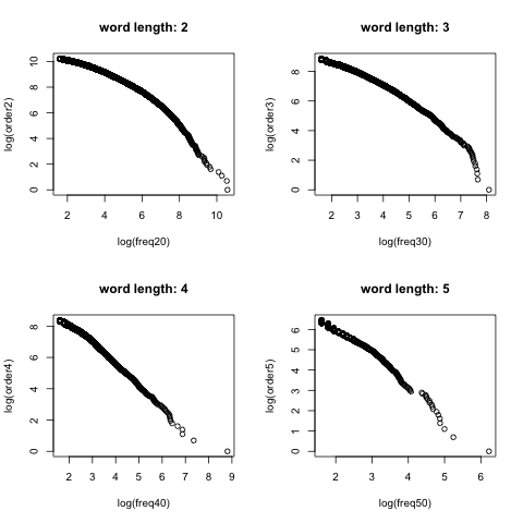
In theory, the first set of plots should look roughly linear. Here, that only becomes barely visible when words are grouped in sets of five by character length. Looking at the top 50 words in those groups, that apparent linearity seems to be driven more by English words than by Chinese ones. That raises a possibility: maybe the part of the corpus that resembles Zipf behavior is the portion shaped by heavy English usage on Weibo.
Here are some high-frequency examples from that group:
     zynga 发展中国家      happy      phone
       504        189        148        131
     webos      china 南京大屠杀      party
       130        125        119        108
     gmail      world      store      style
       106        104         98         98
个人所得税      ilook      never      there
        93         90         89         88
     gucci 高尔夫球场      touch      adobe
        81         79         59         57
     weico      weibo      hello      rovio
        57         56         53         53
     heart 印度尼西亚      icann      green
        50         49         49         47
     belle      kitty      leave 人民检察院
        46         45         45         44
原教旨主义      first      light 毛泽东思想
        44         44         44         43
中国科学院      black      david      kevin
        42         42         42         42
     brian      yahoo 中央气象台      nexon
        41         41         40         40
     nexus      apple      muddy      still
        40         39         39         39
     would      ralph
        39         38
But once the segmentation focuses on two-character and three-character words, Chinese vocabulary dominates. And that is exactly where the distribution departs most clearly from Zipf’s law. Instead of a straight-line relationship, it looks more like a parabolic curve.
Two-character words:
中国  腐败  城管  一个  北京  微博  问题  政府
38951 37655 28787 24242 15834 14984 12972 12651
 社会  今天  美国  国家  工作  公司  经济  已经
11418 11310 11264 11261 10326  9722  8402  8227
 现在  时间  表示  事件  香港  发现  世界  发生
 8222  7941  7913  7755  7710  7466  7258  7196
 进行  知道  人员  安全  生活  目前  新闻  调查
 7189  7184  7077  7032  6985  6916  6901  6378
 记者  今年  孩子  市场  官员  昨天  事故  企业
 6043  6037  6034  5944  5919  5809  5748  5706
 看到  图片  朋友  部门  视频  成为  全国  认为
 5614  5587  5572  5496  5440  5386  5370  5339
 大学  媒体
 5317  5219
Three-character words:
北京市 越来越 房地产 嫌疑人 公安局 老百姓 互联网
  3266   2122   2074   2033   1928   1913   1804
公务员 候选人 联合国 公安部 人民币 电视台 消费者
  1789   1747   1728   1715   1657   1620   1577
亿美元 负责人 委员会 国务院 铁道部 办公室 哈哈哈
  1515   1514   1513   1457   1417   1243   1243
进一步 中纪委 第一次 派出所 开发商    ceo    the
  1241   1213   1125   1099   1096   1090   1068
俄罗斯 幼儿园 临时工 董事长 发言人 意味着 机动车
  1054   1006    982    952    916    902    897
利比亚 大学生    you 万美元 全世界 新华社 朝阳区
   821    798    796    781    766    764    762
领导人 身份证 志愿者 一个月 总经理 自行车 发布会
   750    741    717    705    688    661    651
奢侈品
   642
Does removing stopwords explain the mismatch?
A natural objection is that high-frequency function words were removed, and that operation alone might break Zipf’s law.
That objection is fair as far as it goes. If the original corpus did follow Zipf’s law, then removing frequent stopwords would indeed disrupt the constant (C). Once the ranking is shifted upward, the values at the front should become smaller. But that effect should not force the later part of the curve downward in the same way. If the underlying pattern still held, the tail should gradually approach the constant instead of collapsing away from it.
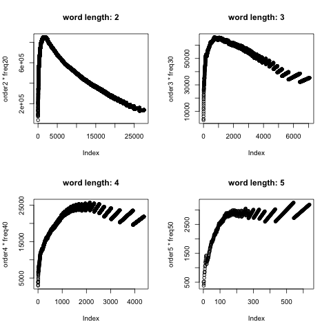
That is where the second set of plots matters. If the Weibo corpus followed Zipf’s law, the graph of (r \times f) should be roughly flat. Instead, it forms a hump—steep on the front side and more gradual on the back.
So the next question becomes obvious: what words are sitting near that peak?
Two-character words near the peak:
人心 阻止 一套 原文 随便 展开 男性 下次 无能 征集
 421  442  422  443  420  643  421  442  422  441
中方 轻松 手中 名人 走红 审判 借贷 滋生 水果 早安
 423  443  420  421  425  442  422  426  643  423
团购 森林   lt 债务 买房 观众 咖啡 环卫 遭到 警告
 642  441  641  640  420  639  443  440  638  421
嘉宾 城区 火锅 争取 选项 转型 原本 姐姐 震惊 角色
 425  442  422  426  423  448  444  441  424  420
军事 欧元 好多 好处 富人 商务 会长 有所 沉默 真心
 443  643  440  421  425  641  422  640  442  445
Three-character words near the peak:
执行官 侦查员 著作权 原材料 总公司    see 男朋友
    91     91     91     92     84     63     91
徐家汇 一口气 知情人 婴幼儿 交易日 信息化 小金库
    90     92     84     63     91     90     92
针对性    lte 写字楼 中文版    lee 银行家 直辖市
    84     81     63     89     80     88     83
专卖店 孙悟空 多一些 太阳能    tot 中南海 微生物
    62     63     91     90     61     81     92
抑郁症 手续费    fbi 自己人 小学校 新街口 一周年
    84     89     80     64     62     83     88
尼古丁    gif 从业者 国家队 一两个 演播室 芝加哥
    63     61     91     90     81     84     71
星期六 玉泉营 想象力 生产力 小博士 十多年 科技界
    80     64     87     92     62     89     63
债权人
    60
Staring at those lists does not immediately reveal a clean explanation. Still, one intuition seems worth keeping.
The product of frequency and rank may work as a rough measure of a term’s influence inside the corpus. In text collections that do follow Zipf’s law, the most influential words would simply be the highest-frequency ones. But those are often the least useful terms analytically, which is why routine NLP pipelines usually remove them.
Once a corpus does not follow Zipf’s law—and once high-frequency stopwords are already filtered out—the question becomes different: how do you find representative terms? The terms you want cannot be too common, because then they become generic noise, but they also cannot be too rare, because then no stable pattern emerges.
By that logic, words with large (r \times f) values may be especially interesting. They are not huge in scale, yet they may differ sharply across groups, and that difference could easily get diluted when Weibo is treated as one broad pool of everyday discussion.
A tentative takeaway
Several points stand out from this experiment:
- Even after removing high-frequency stopwords, the Weibo environment—especially Chinese-language usage—does not appear to fit Zipf’s law very well.
- In Chinese corpora, the hump-shaped pattern in frequency times rank may offer a way to identify comparatively influential keywords within groups.
- The mixture of Chinese and English on Weibo is not a minor detail; it materially affects the distribution.
- There is plenty of room to dig further.